
MATHEMATICS OF NEURAL NETWORKS
The Mathematics of Neural Networks infographic describes the mathematics concepts and algorithms use in neural networks.
- What mathematics is used in neural networks?
- How does it help a neural network learn
- Where does it fit in the curriculum?
See Gadanidis, Li, & Tan (2024)
See also:
- Understanding Neural Networks infographic
- Munchable Matrices graphic story
- Transformative Matrices graphic story
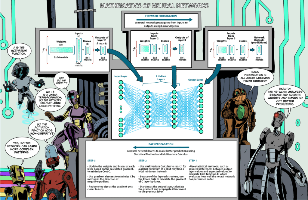
FORWARD PROPAGATION
A neural network is a digital “machine” that is able to learn.

TRAINING A NEURAL NETWORK
A neural network learns by being trained on a set of data.
For example, if the goal is for the network to learn to recognize digits 0-9, it may be trained using numerous variations of digits 0-9, available from the MNIST database.
A sample of this data is shown below.
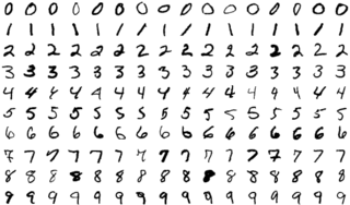
INPUTS TO A NEURAL NETWORK
The training data shown above are the inputs to the neural network.
Such inputs are fed to the second layer of the neural network.
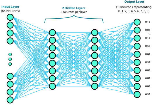
The second layer predicts what weights and biases may be assigned to the inputs, applies the weights and biases, and activation function, and passes the adjusted values to the next layer.
This process continues until the output layer (or last layer).
This process, from input to output, is called forward propagation.
APPLYING WEIGHTS & BIASES TO INPUTS

The image on the right shows how weights (w) and biases (b) are applied inputs (x).
This results in wx + b.
Notice that wx involves the multiplication of 2 matrices.
- w (weights) is an 8×64 matrix
- x (inputs) is a 64×1 matrix
- Their product (wx) results in an 8×1 matrix
- Then the 8×1 biases (b) matrix is added to get wx + b.
Biases adjust neuron values up or down, so they may meet a certain threshold.
APPLYING AN ACTIVATION FUNCTION
Since wx + b is a linear transformation, the network can only learn linear patterns.
To add non-linearity, an activation function (f) is used, resulting in f(wx + b).

This way, the network may learn more complex patterns.

FORWARD PROPAGATION
The process of applying weights, biases and an activation function is repeated in each layer, until the output layer.
This process is called forward propagation.

BACKPROPAGATION
In its training stage, the network compares the difference between predicted and actual values and, through the process of backpropagation, adjusts the weights and bias of each neuron to improve the network’s predictions.
STEP 1: Calculate the cost function
In its training stage, the neural network uses statistical methods (such as squared differences between predicted and expected values) to calculate its cost function C (or error function).
STEP 2: Find the minimum of the cost function
The neural network, in its attempt to minimize its error, searches for the minimum or lowest value of the cost function C.
If only 3 variables are involved, the graph of C would be three-dimensional, and it may look as shown below. However, neural networks use cost functions with many more variables, which cannot be visualized in this way. The variables represent the various weights and biases used by the network.

The lowest points of the valleys in this graph represent all the local minima. That is, they represent the points where the cost or error of the network is the lowest.
The deepest valley is where the global minimum is located, and this is what the backpropagation process is attempting to find.
The neural network uses multivariate calculus to analyze the cost function C. It tracks gradient descent, that is, it moves in the direction of decreasing slope, searching for locations where the slope is zero. In other words, the network searches for the global minimum of C, although it may instead find a local minimum.
2D Python animation
View the animation of the tangent moving along the curve:
- When is the slope of the tangent positive?
- When is the slope of the tangent negative?
- When is the slope of the tangent zero?
3D Python animation
View the animation:
- Which is the lowest point?
- Does the ball always find the lowest point? Why?
See the Python code
Binder
Google CoLab [>18 years old or district license]
STEP 3: Update weights and biases
As the network backpropagates to each layer, it updates the weights and biases.

TRAINING A NEURAL NETWORK
There are various methods to implement neural networks, with the Python programming language being most popular.
PROGRAMMING LIBRARIES
Through Python, various programming libraries are available, which contain ready-made methods for popular AI algorithms and techniques. PyTorch is one example of such libraries, which is fairly easy to use and lends itself well to prototyping.
Thanks to such libraries, it is possible to start training a neural network without much knowledge of the underlying mathematics.
Due to the simplicity of this implementation, the neural network’s accuracy is quite poor.

Simple Digits Classifier
This introductory notebook introduces the basic skeleton for using PyTorch for machine learning. We use the UCI ML hand-written digits data sets, which consist of 1,797 images of 8×8 grayscale digits from 0 to 9. We walk through loading the data set, preparing it for PyTorch, building a basic neural network, and then training and evaluating it on the data set. We provide various visualizations as well.
What to do next to improve the neural network’s accuracy is not always obvious, demonstrating the importance of understanding the underlying mathematics.
See the Python code
Binder
Google CoLab [>18 years old or district license]
Walkthrough of Simple Digits Classifier
by Jonathan Tan, Western University
VIDEO Timeline
- Notebook details
- 1:00 — Accessing the notebook
- 2:20 — How to use Python imports
- 5:40 — UCI data set
- 12:30 — Building the network
- 21:56 — Training the network
- 28:47 — Evaluating the network
- 36:27 — Modifying the notebook and next steps
IMPORTANCE OF MATHEMATICS
In our example, we want the neural network to output a 1 for the correct digit and 0 for the rest to demonstrate a confident and correct prediction.
To train it, we take the squared error between this and the network’s output as a cost function. This seems reasonable, but our model doesn’t perform quite well.
Instead, a better cost function is borrowed from information theory: the cross-entropy loss function. This function is more appropriate for working with probability distributions, as in our classification task. If we had a different task, such as predicting the cost of a house, we might look to a squared-error cost function again.
Improving the Classifier
As the performance of the classifier in the previous notebook is quite poor, in this notebook, we explore various avenues for improving the performance. We try and evaluate things such as changing the data set, modifying the network structure, and using a different cost function.
See the Python code
Binder
Google CoLab [>18 years old or district license]
WHAT DID YOU LEARN?

- What did you learn about the mathematics of neural networks?
- What was most interesting to you?
- What surprised you?
- What else do you want to know?